Binomial Model
Import modules
Import the required distributions:
Binomial: The assumed model likelihoodBeta: Prior forBinomialdistributionBetaBinomial: The posterior predictive distribution
and the functions:
binomial_beta: get the posterior distribution from data and priorbinomial_beta_posterior_predictive: get the posterior predictive
from conjugate.distributions import Beta, Binomial, BetaBinomial
from conjugate.models import binomial_beta, binomial_beta_posterior_predictive

import matplotlib.pyplot as plt
Observed Data
Generate some data from the assumed likelihood
N = 10
true_dist = Binomial(n=N, p=0.5)

# Observed Data
X = true_dist.dist.rvs(size=1, random_state=42)
Bayesian Inference
Get the posterior and posterior predictive distributions
# Conjugate prior
prior = Beta(alpha=1, beta=1)
posterior: Beta = binomial_beta(n=N, x=X, beta_prior=prior)

# Comparison
prior_predictive: BetaBinomial = binomial_beta_posterior_predictive(
    n=N,
    beta=prior,
)
posterior_predictive: BetaBinomial = binomial_beta_posterior_predictive(
    n=N,
    beta=posterior,
)
Additional Analysis
Perform any analysis on the distributions
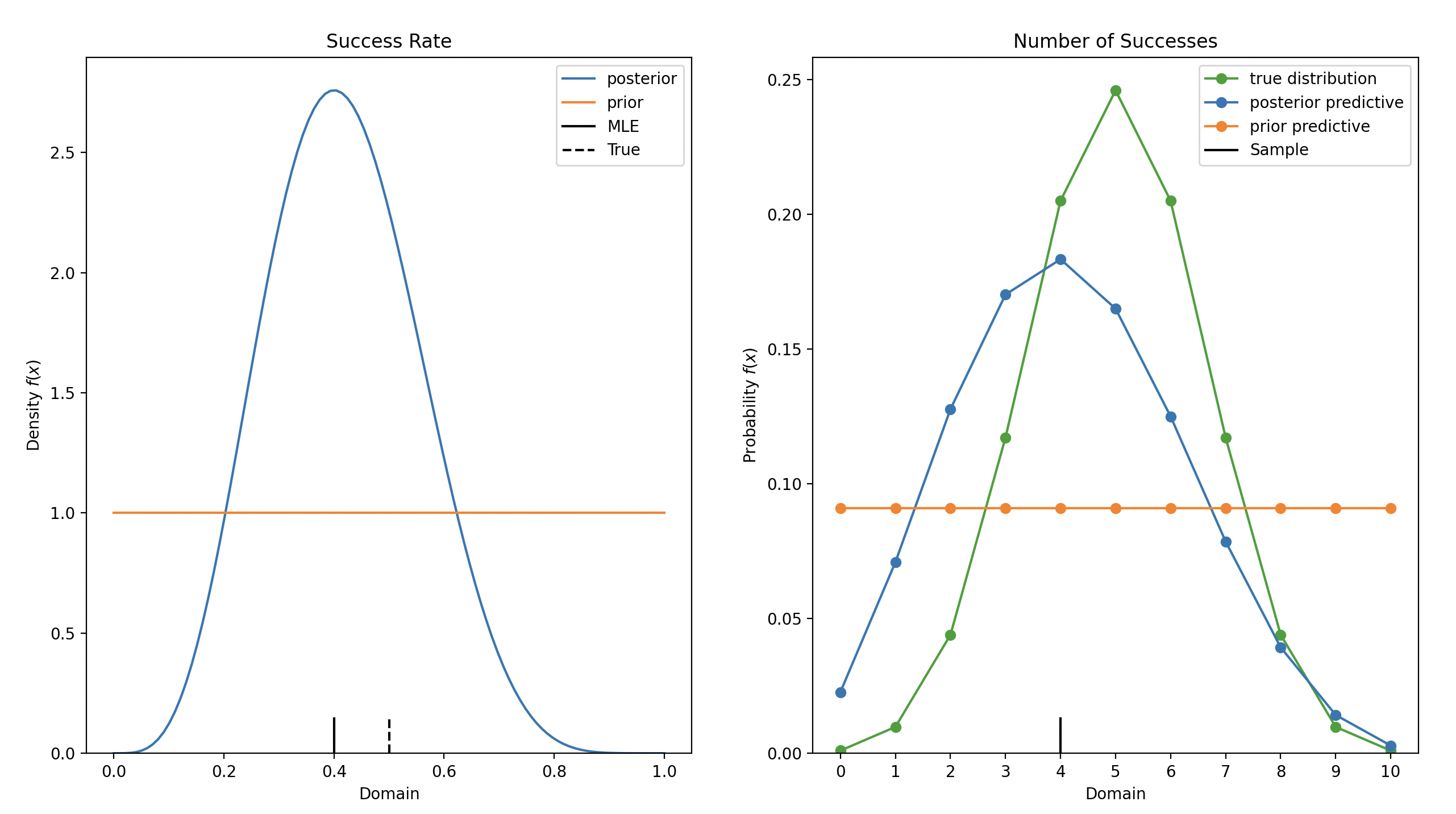
# Figure
fig, axes = plt.subplots(ncols=2, nrows=1, figsize=(8, 4))

ax: plt.Axes = axes[0]
posterior.plot_pdf(ax=ax, label="posterior")
prior.plot_pdf(ax=ax, label="prior")
ax.axvline(x=X/N, color="black", ymax=0.05, label="MLE")
ax.axvline(x=true_dist.p, color="black", ymax=0.05, linestyle="--", label="True")
ax.set_title("Success Rate")
ax.legend()

ax: plt.Axes = axes[1]
true_dist.plot_pmf(ax=ax, label="true distribution", color="C2")
posterior_predictive.plot_pmf(ax=ax, label="posterior predictive")
prior_predictive.plot_pmf(ax=ax, label="prior predictive")
ax.axvline(x=X, color="black", ymax=0.05, label="Sample")
ax.set_title("Number of Successes")
ax.legend()

plt.show()