Conjugate Models

Bayesian conjugate models in Python

Installation

pip install conjugate-models

Features

• Connection to Scipy Distributions with dist attribute
• Built in Plotting with plot_pdf and plot_pmf methods
• Vectorized Operations for parameters and data
• Indexing Parameters for subsetting and slicing
• Generalized Numerical Inputs for inputs other than builtins and numpy arrays
• Unsupported Distributions for sampling from unsupported distributions

Supported Models

Many likelihoods are supported including

• Bernoulli / Binomial
• Categorical / Multinomial
• Poisson
• Normal (including linear regression)
• and many more

Basic Usage

1. Define prior distribution from distributions module
2. Pass data and prior into model from models modules
3. Analytics with posterior and posterior predictive distributions

from conjugate.distributions import Beta, BetaBinomial
from conjugate.models import binomial_beta, binomial_beta_posterior_predictive

# Observed Data
X = 4
N = 10

# Analytics
prior = Beta(1, 1)
prior_predictive: BetaBinomial = binomial_beta_posterior_predictive(n=N, beta=prior)

posterior: Beta = binomial_beta(n=N, x=X, beta_prior=prior)
posterior_predictive: BetaBinomial = binomial_beta_posterior_predictive(n=N, beta=posterior) 

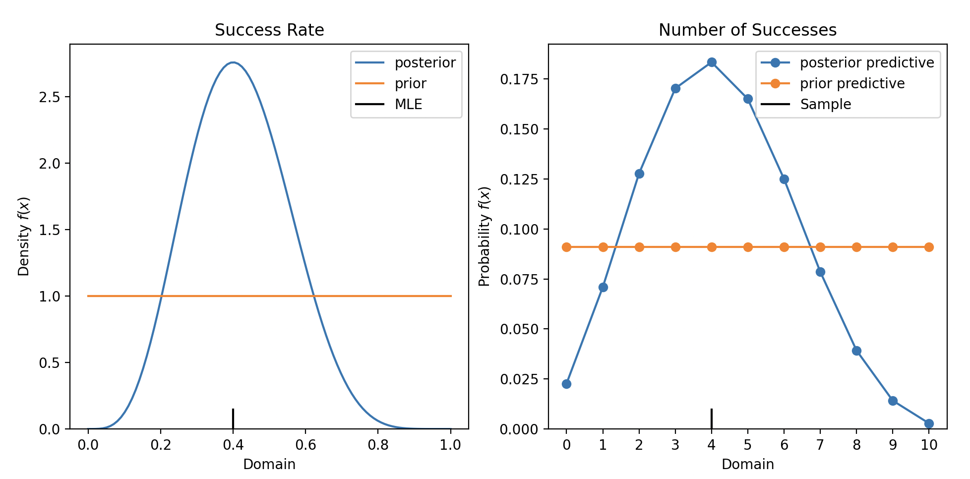
From here, do any analysis you'd like!

# Figure
import matplotlib.pyplot as plt

fig, axes = plt.subplots(ncols=2)

ax = axes[0]
ax = posterior.plot_pdf(ax=ax, label="posterior")
prior.plot_pdf(ax=ax, label="prior")
ax.axvline(x=X/N, color="black", ymax=0.05, label="MLE")
ax.set_title("Success Rate")
ax.legend()

ax = axes[1]
posterior_predictive.plot_pmf(ax=ax, label="posterior predictive")
prior_predictive.plot_pmf(ax=ax, label="prior predictive")
ax.axvline(x=X, color="black", ymax=0.05, label="Sample")
ax.set_title("Number of Successes")
ax.legend()
plt.show()

Too Simple?

Simple model, sure. Useful model, potentially.

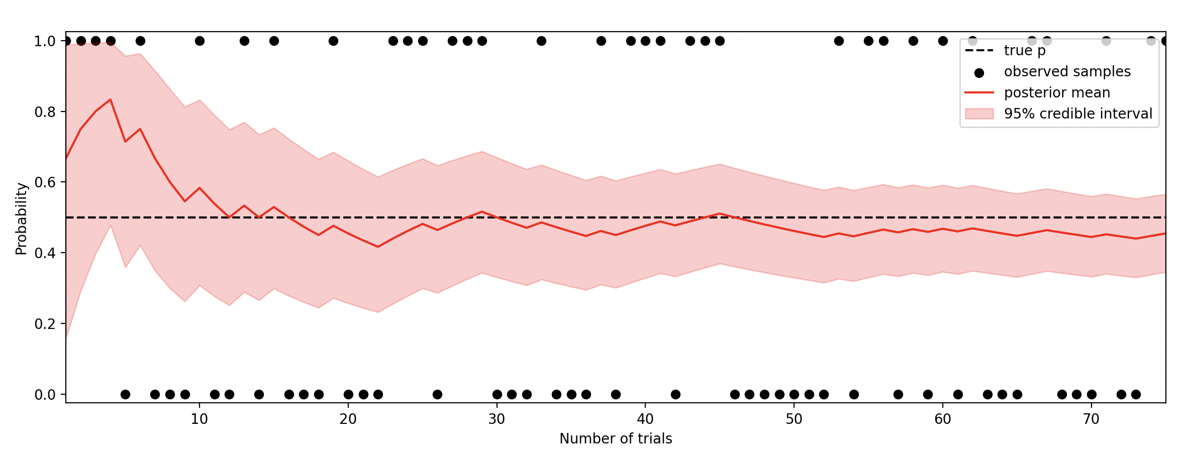
Constant probability of success, p, for n trials.

rng = np.random.default_rng(42)

# Observed Data
n_times = 75
p = np.repeat(0.5, n_times)
samples = rng.binomial(n=1, p=p, size=n_times)

# Model
n = np.arange(n_times) + 1
prior = Beta(alpha=1, beta=1)
posterior = binomial_beta(n=n, x=samples.cumsum(), beta_prior=prior)

# Figure
plt.plot(n, p, color="black", label="true p", linestyle="--")
plt.scatter(n, samples, color="black", label="observed samples")
plt.plot(n, posterior.dist.mean(), color="red", label="posterior mean")
# fill between the 95% credible interval
plt.fill_between(
    n, 
    posterior.dist.ppf(0.025),
    posterior.dist.ppf(0.975),
    color="red",
    alpha=0.2,
    label="95% credible interval",
)
padding = 0.025
plt.ylim(0 - padding, 1 + padding)
plt.xlim(1, n_times)
plt.legend(loc="best")
plt.xlabel("Number of trials")
plt.ylabel("Probability")
plt.show()

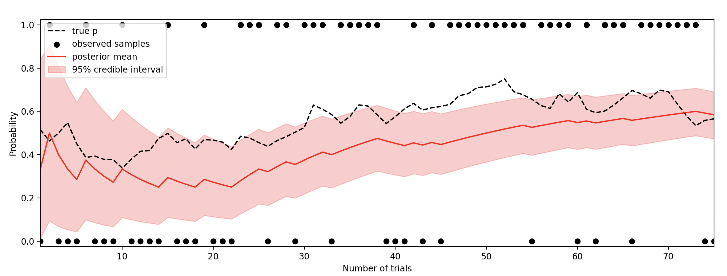
Even with a moving probability, this simple to implement model can be useful.

...

def sigmoid(x):
    return 1 / (1 + np.exp(-x))

p_raw = rng.normal(loc=0, scale=0.2, size=n_times).cumsum()
p = sigmoid(p_raw)

...

Resources

• Conjugate Priors